The Nuclear Equivalent to the War on Terror

All the money spent in Iraq and Afghanistan represents resources destroyed. As of September, 2021, a study from Brown University estimates the US has spent $8 Trillion.

https://www.brown.edu/news/2021-09-01/costsofwar

But, that's just money. How much, in terms of real resources, does $8  Trillion US, $8000 Billion US, represent?  Let's do residential. Medial value of a house in the United States is $140K. (2010)

 That's about 7 million houses. The equivalent value of 7 million houses which is not being invested, rather is being destroyed in warfare. 7 million houses which are not being built. 7 million houses figure 4 persons per house, 28 million people. So the residential equivalent of a several very large cities has being leveled. This kind of calculation has been done, more accurately and in greater detail, both nationally and for the share of one's locality, and can be found by searching in say: 'cost of the war in Afghanistan'. Nobody is being hurt though. But: Let's look at it in terms of man lives. Average GDP per worker is roughly, $14T/140M in the labor force, these days gives $100K per worker. So the cost is 10M man years. Figure 40 years productive life: $4M per life. So: $1000B/$4M = 250K lives. So the war on Terror has destroyed the lifetime production of 250 thousand men. Economically speaking, these are the casualties the US has sustained. Let's check the nuclear option. When you nuke a city, you destroy only half the lifetime productive capacity of the population (half has already been contributed) so DOUBLE the number of people killed. Figure 500K. Note we are now considering everyone in our city as labor or potential labor. Now the total capital of the US is about $50T. Divide by total people (300M) and you get about $170K per person, of physical capital, that is houses, factories, offices, roads, utilities, etc. they occupy and use. An interesting number in its own right. But we'll use $200K. So that's $100B worth of capital our 500K people occupy and use. (200K x 500K.) Figure $100B to be the equivalent of 25K man lives. ($100B/$4M = 25K man lives.) We subtract 25K man lives because we're blowing up their productive lives equivalent in material destruction, giving 475K. We're subtracting it because we don't want to count it twice. But we see that counting the actual material that is blown up is just a small correction. We can just as well ignore it, given the approximate nature of all our numbers So, roughly, the War on Terror has, so far, cost the economic equivalent of the total destruction of a city of 500 thousand people. Give or take. That's everyone and everything in it. That's a lot of terrorism. Of course ‘economic equivalent’ does not include pain and suffering. Or cleanup. Most of the numbers we've used understate the answer. One can argue that we understate the earnings per man life, but don't forget capital is spent on the individual at both the beginning and end of his life, so the net contribution of a person to society is probably considerably less than 40 years of labor. By our calculations 9/11 resulted in the destruction of something under 5 thousand man lives of production. The War on Terror is, it seems, a rather disproportionate response. But then, one can always claim WWII was a disproportionate response to Pearl Harbor.

Does Holiday Shopping Boost the Economy?

Does the holiday shopping season boost the economy? Or does it matter? Or is the economy actually harmed by it?

Or does it depend on the state of the economy? 

By tradition, Black Friday is when retailers, when their sales are summed out over the year, first start netting a profit. ( If so, we can figure that retailers net on average over 10% profit, figuring total sales over the month of December to be even slightly more than the average month.)

But we follow the money.  First, consumers only have so much to spend over the course of a year. No matter how their spending is distributed, it doesn’t affect how much they have to begin with, and that is what limits how much they have to spend. If they spent less during the holiday season, they would have more to spend during the rest of the year. From that point of view, the holiday shopping season doesn’t affect the economy at all, except to make its activities uneven.  

However, suppose the season motivates people to take on a larger debt burden than they otherwise would.  This in the long run might lead to a decrease in growth in the real economy.  This is the consequence of the fact that, when we subtract the cost of borrowing, that is the interest paid by the consumer, the consumer has less to spend in the long run.  Of course, that interest is someone else’s income.  Since borrowing is by the poor from the rich, and the rich spend a lower percentage of their income, the implication is that total demand is reduced, and will grow more slowly. And so the economy with it. Also the distribution of wealth is changed, further concentrated on the rich, and this is not a good thing.

Supposing instead, on average, the existence of the holiday shopping season induces people to save more. Then in the long run, they would have more to spend, because of the interest, and this would lead to greater demand, and increased growth.  In the long run. But evidence doesn’t suggest increased savings to be the case. 

There is the additional cost of increased competition, the cost of stores open on holidays, and longer hours, the increased burden on infrastructure.  This additional destruction of resources makes us all a bit poorer.

There is the time and opportunity cost to consumers, waiting for their place in line, when they could be doing something more productive, and that makes them, and all of us, poorer.

If the economy was at full capacity before the holiday season, the increase in demand might lead to production bottlenecks, and inflation. This might be harmful. In a slack economy, it is hard to see this would be a problem, and might temporarily help the employment situation.  However, it shouldn’t affect the employment averaged over the course of a year.   

Anyway, at best, in net, we conclude the holiday shopping season has a slightly negative effect on the total economy.  Further, the compromising of the holiday of Thanksgiving, (and some might argue of Christmas also,) in the unseemly pursuit of profit, and the induced and equally unseemly pursuit of bargains, must be counted a social negative, and evidence that we cannot evaluate the well being and progress of a society merely by the measurement of economic factors.

Oligopsonies in an Economy

Our study of oligopsonies will follow our study of oligopolies, which the reader will find helpful to refer to.  Oligopsonies are another example of the macroeconomic effects of microeconomic processes.  The derivation is based on the idea of the kinked supply curve, which may be out there but doesn’t seem easy to find. That oligopsonies create market distortion is well known. 

We discuss competitive oligopsonies, where collusion is not necessary.

For your convenience a little background. Oligopsonies are ubiquitous. It seems many markets evolve into them.  Although consumers do not directly experience them, (except in labor markets,) they may often occur as the back end of oligopolies. One oligopsony is the fast food industry, which forms an oligopsony to meat sellers.   It also forms an oligopoly to cheeseburger buyers.  (A suggested word is oligonomy. See: http://activism101.ning.com/profiles/blogs/oligonomy-defined) The factors, goods or services which go into the oligopolist’s product, which are unique to an oligopoly, face oligopsony. 

Other examples of (non-labor) oligopsony are 1:  Cocoa market, where three firms buy the vast majority of cocoa.  2:  American tobacco market, where three cigarette makers buy 90% of all tobacco grown in the US. 3: the culinary herb market.  

 The various drug cartels  may also constitute a oligopsony for drug producers, and an oligopoly for drug users.

The characteristics of an oligopsony are 1:  It consists of a relatively few, relatively large, buyers.  2:  Each firm is big enough to affect the others. That is, the prices each firm pays affect the prices paid by the other firms. 3:  The goods or services they buy are similar or identical.  4:  There are barriers to entry, such as initial capital costs. A firm needs to be capitalized to have a profitable use for what it buys.  

Those not interested in the derivation may jump ahead to the discussion at the conclusion.  Those interested might also find discussions on monopsony helpful.  Here’s one:

http://www.youtube.com/watch?v=gKUvnFOu02U

Since oligopsonies are buyers instead of sellers, instead of a kinked demand curve, the individual oligopsonist faces a kinked supply curve, S, which is also his average cost curve AC, This is the price he pays for his goods,.  Diagram 1 shows this supply curve for a particular oligopsonist.  The oligopsonist wants to buy at the kink, a which is at some price p_a, which is really determined by the market, and some quantity q_a, which is determined by other factors, which we will discuss in the conclusion. In any event, the kink at which he buys is at a lower price than the price at competitive equilibrium, (around e) and a smaller quantity.  His total cost is price times quantity bought, or p_a x q_a.

Why does he want to buy at price p_a?  If he lowers the prices he offers below p_a, to p_b, hoping to save money, none of his competitors will follow.  Since his prices are below theirs, and because they are all buying the same of similar goods, sellers will go to his competition, and he will lose market share. (Note the assumption that there is not so much to sell, that many buyers will have to come to him, anyway.) If the price he offers goes down a little, the quantity of goods he is able to buy will go way down, to q_b.  This is the characteristic of an elastic supply curve.  As you move down the curve, the quantity the oligopsoninst is able to buy goes down.  Since these goods are factors of production, the oligopsonist can no longer produce at the same scale as before, cutting into his profit margins. 

Suppose instead he raises the prices he offers, from p_a to p_c, hoping to gain market share.  Then his competitors will quickly follow suit, since they don’t want to lose their market share to him.  So he won’t gain market share, he’ll just be buying at a higher price.  He may, however, buy a few more, at q_c, just because his and everybody’s price is higher.   This is characteristic of an inelastic supply curve.  Since his costs per unit are higher, his profit margins are likely to be slimmer, since he won’t be producing appreciably more of his product.  

Now for a firm to maximize profits, its marginal costs, MC, must equal its marginal revenue product, MRP, which is also its demand curve, D.   This is always the case, but what does this mean?    The marginal revenue product, MRP, is the use the oligopsonist gets out of the next unit he buys.  This is (mostly) a decreasing function because of the law of diminishing returns.  This decreasing function is what we show in the diagram. (But we say mostly because consider our restauranteur buying labor. In his case the first worker is useless. He is simply not enough to run a restaurant.   So his MRP for labor starts at zero and  increases until it reaches some maximum, then decreases steadily, since further workers start getting in each other’s way and contribute an ever decreasing amount to his total profit.  Most analyses ignore this, and you can, too.  For goods, the MRP is  usually a simpler, a steadily decreasing function, although again economies of scale would make it first go up.)

Marginal cost is the increase in cost that results from buying one more unit.    For imperfect competition, as we have in the case of oligopsonies, MC is always more than the average cost, AC.  (AC is also the supply curve, S, remember.)  This is because when you buy more units, you have to buy them at a higher price, but you have to buy all your units at that higher price.   So if the firm buys 4 units for $60 and has to pay $90 for 5 units, then the marginal cost of the fifth unit is $30.   The average cost however, is $18, and lower than the marginal cost.

Profit is maximized when MRP = MC because when MC is greater than MRP, it costs more to buy the next unit than you get use out of it.  With the figures we used, you would buy 4 units for $60, get use out of them for $100, (manufacture some things you can sell for $100, say,) and make $40 profit.  If you were maximizing profit, you wouldn’t then buy 5 units for $90, having use of them for $125, and only make $35 profit. 

See Diagram 2.  The marginal revenue product MRP curve is the downward sloping line.

With the kinked supply or AC curve, the MC curve is very strange.  The AC_L and the MC_L curve, the curves below the kink, both start at the same point on the axis, (in the direction where the arrows come together,) but the MC_L curve ascends more steeply, twice as steep, it turns out. When they reach the kink, however, the MC_U and AC_U curves, the curves above the kink, also extend from a point on the axis, (much lower on the axis) in the direction of the dotted arrows, so the MC_U curve, being twice as steep as the AC_U curve, is much higher than the MC_L curve at the kink. (The upper and lower labels are for convenience.  They are just different parts of the same line.)

What is important is the green line, the marginal cost MC_V curve at the kink, which is vertical.  Now since, when we maximize profit, MRP = MC, when ever MRP crosses the green MC_V line, (at the star,) the profit maximizing quantity qa and price pa are going to stay the same.  See Diagram 3.  The firm, whether its marginal revenue product curve is MRP₁, or MRP₂ or MRP₃  is going to want to buy the same amount qa, and pay the same price pa.  This will maximize its profit.

Conclusion:  Since firms in oligopsonistic competition tend to be locked in to price, they must find other ways to compete, and maintain or gain market share.  The leader of a drug cartel, for instance, might resort to escalating levels of violence to secure market share.   (We make the casual observation that one need look no further than oligopsony, (and oligopoly,) pricing to deduce a cause for Keynesian ‘price stickiness.’  In an economy rife with oligopsony we would expect many points of price, and quantity, fixedness, making deflation a uneven and problematic process.) 

Consider MRP₃ in Diagram 3.  The oligopsonist would not want to lower marginal revenue product any more, through non-price competition, because then his profit maximization would occur at a price lower than p_a, and he would lose market share.

However, the opposite can also happen.  Since price is, with in a range, independent of costs, the oligopsonist may decide to increase  his MRP, use what he buys more efficiently, and so increase his profit that way. 

Oligopsonies do not consist of identical or identically sized firms, with identical shares of the market. The quantity a particular oligopsonist buys at is determined by historical factors, and his ability, or inclination, to compete in ways which do not affect the price he offers for the goods or services he buys. Working conditions, for instance, may be one way a labor oligopsonist may attract a better class of laborer, enhance his MRP, and so his profits. Historical factors, for instance, most notably their activities during the period their industry was more competitive and open, determined the relative sizes of Wendy’s, McDonald’s and Burger King before they filled the market and became an oligopsony.  Decisions since have changed their relative sizes and profitability.   

Another point is that, unlike perfect competition, firms of various efficiencies can co-exist in an oligopsony, operating at differing capacities and different economies of scale, each firm collecting its particular degree of profit.  And unlike perfect competition,  much of this profit is extra-normal.  Even an inefficient firm can make an extra-normal profit.

What other things might we expect?  Well, we would expect the transfer of some producer surplus to the buyer, in the form of his extra-normal profits. (The oligopsonistic buyer is seldom the ultimate consumer.) Consider that oligopsonies are becoming economically pervasive.  Each of these oligopsonies extracts its rent, transferring resources from producers, to the oligopsonists.  Indeed, to simplify considerations, let us just model the entire economy as two tiers, consisting of an oligopsony and those who sell to it.  Consider first perfect competition, where the economy was efficient and in balance, Diagram 4. 

 Supply equals demand and the equilibrium point e, and surplus is divided between seller and buyer. With oligopsony, Diagram 5, there is a net transfer of surplus from the seller to the oligopsonists. (the greenish-yellow box)  In the real economy, this would be manifest as lower producer profits.  We would thus expect a gradual decapitalization of  producers.  In a labor oligopsony, we would expect decrease in the welfare of labor, as the increase in the income of the oligopsonist has to come from somewhere. 

 

Efficiency has also declined because an oligopsony buys less than the competitive equilibrium production, at a lower price creating what is called deadweight loss:  The blue triangle in Diagram 5.  (I’m not sure if the blue triangle is exactly the right one, as I am not sure the exact location of the point of competitive equilibrium in the absence of oligopsony.) That is, the economy is producing less than it would otherwise, perhaps less than it needs to.  In a labor market, this would imply increased levels of unemployment.  For instance, since the public sector also supplies the private sector, as the private sector becomes increasingly organized as oligopsony, we would expect public sector income, supported by taxes on labor costs, to decrease.  We would also expect, due to dead weight loss, an increasing shortage of public goods.

Oligopoly and the Economy

This is a brief discussion of the effect of oligopolies on an economy. It is an example of the macroeconomic effects of microeconomic processes.   The derivation is based on the idea of the kinked demand curve, developed by Paul Sweezy in the 1950’s. 

Those not interested in the derivation may jump ahead to the discussion at the conclusion. 

Those interested may find the various derivations of kinked demand curve theory on You Tube helpful, and perhaps easier to follow than what I have presented here.  Here’s one:

http://www.youtube.com/watch?v=5BQPx8SL9F4.
You might also find  discussions on monopoly, a simpler case of extra-normal profit, helpful.  Here’s one:
http://www.youtube.com/watch?v=3NMbcfS68IQ&feature=related

And for contrast, perfect competition:

http://www.youtube.com/watch?v=7lhX78vlHSY

We discuss competitive oligopolies, where collusion is not necessary for fixed prices.

For your convenience a little background.  Oligopolies are a common market structure.  Indeed, many markets seem to evolve, or  have evolved, into oligopolies, (or its cousin, oligopsonies,)  They are ubiquitous.

An oligopoly has some of the characteristics of a monopoly, in that its members can charge higher than normal prices and make higher than normal profits.  The particular characteristics of an oligopoly are,  1 It consists of a relatively few, relatively large, sellers  2.  Each firm is big enough to affect the others. 3:  The products are similar or identical.  4:  There are barriers to entry, such as initial capital costs. 

The traditional analysis of oligopolies is that, rather than a normal straight demand curve, they face a kinked demand curve D, which for a particular firm is also their average revenue curve AR.  Diagram 1 shows this demand curve for a particular oligopolist.  The oligopolist wants to sell at the kink, which is at some price p_a, which is really determined by the market, and some quantity q_a, which is determined by other factors, which we will discuss in the conclusion.In any event, the kink is at a price higher than the equilibrium price in perfect competition, and a quantity lower than the equilibrium quantity. Fewer goods are produced, and consumers are forced to pay a higher price for them.

If we were to discuss all the members of this oligopoly, they would each have a separate, though similar, diagram.  The prices at the kink would all be the same, but the quantities at the kink might be different. 

  

Our oligopolist’s total revenue, that is, how much money he takes in, is price times quantity sold, or p_a x q_a.

Why does he want to sell at price p_a?  If he raises his prices above p_a, to p_b hoping to make an extra profit, none of his competitors will follow.  So his prices will be above theirs, and because their products are similar to or identical to his, he will lose some, perhaps many of his customers to them.  If his price goes up a little, the quantity of products he sells will go way down, to q_b so he will take in less money. The area  

p_b x q_b, the money he takes in now, is less than the area p_a x q_a, the money he took in before.  This is the characteristic of an elastic demand curve. As you move up the curve, the quantity sold goes down faster than the price goes up.   

Suppose instead he lowers his prices, below p_a, to p_c,  hoping to gain market share.  Then his competitors will quickly follow suit, since they don’t want to lose their market share to him.  So he won’t gain market share, he’ll just be selling at a lower price, and making less money.  He may sell a few more products, at q_c just because his, and everybody’s, price is lower, but not enough to compensate for the decrease in price.    The area  p_c x q_c , the money he takes in now, is less than the area p_a x q_a, the money he took in before.  This is the characteristic of an inelastic demand curve.  As you go down the demand curve, the price goes down faster than the quantity sold goes up.

Now for a firm to maximize profits, its marginal costs, MC, must equal its marginal revenue MR.  This is always the case, but what does this mean?  Marginal cost is the increase in total cost accrued by the firm for the next unit it produces.  If the firm produces 4 units for $60 and 5 units for $90, then the marginal cost of the fifth unit is $30.

Marginal revenue is the increase in revenue that results from selling one more unit.    For imperfect competition, as we have in the case of oligopolies, MR is always less than the average revenue, AR.  This is because when you sell more units, you have to sell them at a lower price, but you have to sell all your units at that lower price.  So if you sell 4 units at $100 total revenue and 5 units at $120 total revenue the average revenue AR, the price you are selling them at, for 5 units is $24, but the marginal revenue MR for the 5^th unit is only $20.

Profit is maximized when MR = MC because when MC is greater than MR, it costs more to produce the next unit than you get paid for it.  With the figures we used, you would produce 4 units for $60, sell them for $100, and make $40 profit.  If you were maximizing profit, you wouldn’t make 5 units for $90, having to sell them at $120, and only make $30 profit. 

See Diagram 2.  The marginal cost MC curve is the lopsided “u.” When you produce something, costs first go down, savings of scale, then they go up, dissavings of scale.  (Imagine a restaurant.  The first meal is very costly, because of all your fixed costs. As you produce more, each next meal is cheaper to produce, as you use your assets more efficiently, until you reach some minimum.  Then the costs per each additional meal start going back up, because you run out of stove space, people start getting in each others way, etc.) 

With the kinked demand or AR curve, the MR curve is very strange.  The upper AR_U and the upper MR_U curve, the curves above the kink,  both start at the same point on the axis, (in the direction where the arrows come together,) but the MR_U curve descends more steeply, twice as steep, it turns out. When they reach the kink, however, the MR_L and AR_L curves, the curves below the kink, also extend from a point on the axis, (much higher on the axis) in the direction of the dotted arrows, so the MR_L curve, being twice as steep as the AR_L curve, is much lower than the MR_U curve at the kink.  In this diagram, in fact, it is so much lower it is negative, which means MR_L curve is irrelevant.  What is not irrelevant is the fact that, because MR_L is negative, the MR curve which connects the MR_U and MR_L curves,  (green line) crosses the Q axis at the kink.  This means that the quantity of production of maximum revenue (which is where the MR curve crosses the Q axis) and profit maximization (where MR = MC)are at the same quantity, q_a.

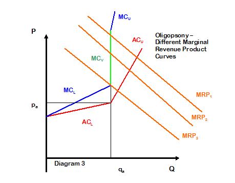
What is important is the green line, the MR curve at the kink.  Now since, when we maximize profit,  MR = MC, when ever MC crosses the green line, the profit maximizing quantity and price are going to stay the same.  See Diagram 3.  The firm, whether its marginal cost curve is MC₁, or MC₂ or MC₃  is going to want to produce the same amount, and charge the same price.  Here this will maximize both profit and revenue.

Conclusion:
 Even in competition, oligopolists can make extra-normal profits.   Firms in oligopolistic competition tend to be locked in to price, so they must find other ways to compete, and maintain or gain market share.  (We make the casual observation that one need look no further than oligopoly pricing (and as we shall see, oligopsony pricing) to deduce a cause for Keynesian ‘price stickiness.’  In an economy rife with oligopoly we would expect many points of price, and quantity, fixedness, making deflation a uneven and problematic process.)  The owner of a service station, for instance, locked in competition with 3 other service stations at an intersection, might, to attract more customers, initiate full service, or add a convenience store or coffee shop.  He might do this, raising his costs, until the marginal cost curve was something like MC₃ in Diagram 3.  The oligopolist would not want to raise costs any more, because then his profit maximization would occur at a price higher than p_a, and he would lose market share.

However, the opposite can also happen.  Since price is, with in a range, independent of costs, the oligopolist may decide to shave costs, cut corners, and so increase his profit that way.  Were an industry to do this, we would have a situation like the American auto industry in the 60’s and 70’s, before imports began to significantly impact on their market.

Oligopolies do not consist of identical or identically sized firms, with identical shares of the market. The quantity a particular oligopolist sells at is determined by historical factors, and his ability, or inclination, to compete in ways which do not affect the price.  Historical factors, for instance, most notably their activities during the period their industry was more competitive and open, determined the relative sizes of GM, Ford, Chrysler, and American Motors, back when they constituted an oligopoly.  Foreign Competition and decisions since have changed their relative sizes and profitability.   

Another point is that, unlike perfect competition, firms of various efficiencies can co-exist in an oligopoly, operating at differing capacities and different economies of scale, each firm collecting its particular degree of profit.  And unlike perfect competition, much of this profit is extra-normal, more than the profits we would expect to see from perfect competition, which tends to drive profit to a minimum.

What other things might we expect?  Well, we would expect the transfer of some consumer surplus to the producer, in the form of his extra-normal profits.  Consider that oligopolies are becoming economically pervasive.  Each of these oligopolies extracts its rent, transferring resources from consumers, to the oligopolists.  Indeed, to simplify considerations, let us just model the entire economy as two tiers, consisting of an oligopoly and its market.  Consider first perfect competition, where the economy was efficient and in balance, Diagram 4.

Supply equals demand and the equilibrium point is at e, and surplus is divided between consumer and producer. (Consumer’s Surplus is  exaggerated a bit, to keep the lines the same.  Sorry.)  With oligopoly, Diagram 5, there is a net transfer of surplus from the consumer to the oligopolists. (the greenish-yellow box) 

 In the real economy, this would be manifest as higher corporate profits, and, since most corporate stock is held by the wealthy, an increase in income of the wealthy.  Corresponding to this, we would expect a decrease in the welfare of the rest of the economy, as the increase in income of the wealthy has to come from somewhere.

Efficiency has also declined because an oligopoly produces less than the competitive equilibrium production, at a higher price creating deadweight loss:  The blue triangle.  That is, the economy is producing less than it would otherwise, less than consumers would be willing to buy at the lower, equilibrium, price.  Indeed, the economy may perhaps be producing less than it needs to.  For instance, since the public sector is also supplied by the private sector, as the private sector becomes increasingly organized as oligopoly, we would expect public sector costs to increase disproportionately.  We would also expect, due to dead weight loss, an increasing shortage, and/or a decline of the quality, of public goods.  This includes much of the infrastructure the private sector, the oligopolist, relies on.

What is a life worth?

Well, on the one hand, it is priceless. But from an economic point of view, a life is only worth about $4,000,000. Of that, $2,000,000 is the person’s worth to himself, and any others he provides for. The other $2,000,000 is the person’s worth to the rest of the economy. How much the rest of the economy benefits from his life’s labor. These figures are very rough, the mean, and of course vary greatly from person to person.


But how do we figure? First, we figure a person is only worth to an economy what he contributes to society. So we figure from a labor force of 150 Million we have a GDP of 14 Trillion. Round that to make the annual contribution to the economy per worker an even $100,000. Times say 40 years labor, about the number of years we suppose the average worker to work in a lifetime. $4,000,000. About half of that goes to the worker, about half to the rest of the economy. That’s the mean. The median worker only gets about$1.4M, but the median worker also probably contributes less than $4M. But what about the people who don’t contribute to the GDP? Well, here we’re counting them the same. Perhaps we shouldn’t. After all, someone who is compensated more than he contributes to society has a negative value to society. But we can also figure not all contributions to an economy show up in the GDP.


This has important ramifications. Such a heartless calculation actually suggests important ways individuals, and society, benefit. It means, for instance, that it is beneficial to individuals if we don’t spend too much saving a life. For instance, we wouldn’t want to spend $1 Trillion to save one life. Everyone else would be that much poorer. The economy would be out $999,996,000,000. That’s just dollars, but the equivalent in lives (valued at $4,000,000) is 249,999. It is 499,999 lives if we take the value a life is worth to the rest of the economy. We would be trading that many lives for one life. This is a bad deal for an economy. If it did this too much, it would literally kill itself.

What about pain and suffering? People are not just economic mechanisms. They have feelings. They feel pain. Can we put a dollar value on that? Sure. Let’s say $1 Trillion on a person’s feelings. Would we want to spend $1 Trillion on a person’s life? We just went through that calculation, and the point is the same. It would overvalue that life, and be a bad deal for the rest of the economy, which is to say, everyone else. It wouldn’t be fair. You can spend $1 Trillion to save one life, but you can’t spend $1 Trillion per person on everybody else, to save their lives. In fact, it works out you can only spend less than $100,000 per year per person. On average.

We can look at it this way: The economy exists to save, and is essentially saving, everybody’s lives, all the time. We’re all on life support. And since the average each worker contributes is less than $100,000 per year, that is all we can spend, on average, per person, per year.

This shows that it is important not to overvalue life. A society which takes excess precautions against the loss of life is the poorer for it. In a sense, it is literally killing more people to prevent the loss of fewer.

Hospitals already often use a rule of thumb. Their guideline is, (often) for spending up to $100,000 per year of life extension. This is equal to our total annual contribution to the economy per worker. For instance, consider extending the life of an elderly person. On the one hand, society typically does not gain any benefit. On the other, the elderly person has already contributed his share to society, and in a sense has earned this consideration, as a kind of savings. And it provides an incentive for people to keep working. But the figure of $100,000 per year is probably too high, considering the limits of the current health care system’s ability to supply health care, and the high rents already collected from it, and contributes to the high costs of medicine today. The rents imply that the benefits to the patient are far less than the $100,000 expended, so the actual value of life is lower than the nominal one. Indeed, if we consider the rent to be 40% of the system, that is, 40% is ‘wasted’ compared to the health care systems of other advanced economies, then the actual value of a person-year is $60,000. This suggests an economic value of $2.4M for a life, lower than our calculated value of $4M.


One interesting, if perverse, example of the extreme is the California death penalty, reinstituted in 1978, which has cost $308M per person (13) executed. Indeed, its total cost $4B, is a substantial share of the California deficit. We can make this calculation: $308M divided by $4M is the total destruction of the lifetime production of 77 people. In this case, the state is effectively killing (the productive capacity of) more people than the criminal ever did. From another perspective, the annual cost of $184M is equal to the total annual contribution of 1840 workers to the economy, almost twice as many as are actually on death row. The work of 1840 workers, wasted.

The EPA, now, gives a figure of $7.9 Million for the value of one life, almost twice the total economic value we calculated, or 4 times the net value of a life to the economy. http://thenewamerican.com/tech-mainmenu-30/environment/6013-epa-reevaluates-the-value-of-human-life

Not a very good trade off. Of course, there is also quality of life. Clean air is better than polluted air, even if the polluted air doesn’t kill you.

Regulations impose costs on producers. By not permitting the externalization of costs, (pollution of one sort or another for the EPA) which by the EPA’s calculations, would cause an increase in death (and disease,) things cost more to produce, and these costs are passed on to consumers. But it also results in less of those things being produced, and since resources are consumed in all production, less being consumed. So in the case of environmental regulations, other benefits accrue than just the saving of lives. Resources are conserved, other things which might be expensive to remedy are reduced. Such things might be considered to be included when the value of a life is overestimated.

Undervaluing life has its own costs. Negative externalities, excess pollution, is encouraged. Overproduction of stuff is encouraged. (This could be an argument for undervaluing life, where increasing the amount of stuff is equated to economic progress!) There are more accidents, as insufficient precautions are taken. There is loss of life and quality of life.

Note, when an economy is poorer, the capitalization per person, and what depends on it, the individual’s ability to contribute to society, thus the value of life, is less. Kenya for instance has a GDP per capita of $1600, $66B/41M but a labor force of 18M, so the average economic contribution per worker is about $3700, times 40 years or about $150K over a lifetime, (average life expectancy about 60, but do they have retirement?) so that is the mean economic value of a life, there.

Back to the US:
A child, on the other hand, has the potential to contribute $4,000,000 to society. But society has not yet invested in him. In fact, (our) society, on the average will invest somewhere around $350,000 in raising a child to adulthood, not counting the opportunity cost of parenting. Most of this cost is born by the family, so does not subtract from the $2,000,000 net contribution. A six year old, for instance, has about $70,000 invested in him, by his family: $60,000 direct costs, and $10,000 or so for his first year of schooling, which one way or another is borne by taxes. Now families are not the only ones to pay these taxes, so there is some subsidy of education by the rest of society. This omits cost- the opportunity cost to the self for his education, when, instead of capitalizing in himself, he could be doing something else.

In fact, it could be argued that the only real loss to society is this investment, and not the inferred profits society takes from his labor. And this investment is all society should be insured against. (This argument is also carried out in: http://en.wikipedia.org/wiki/Value_of_life )

Of course, the actual capitalization may be more or less than that figure, depending on the efficiency of parenting and the educational system, and the social system of the community. Much of the cost of the educational system now seems to be going to rent, judging from the reported decline in results. So the actual capitalization is less.

Further consideration indicates that the health care system may be considered part of the capitalization of individuals. Consider a child who needs a $50,000 surgery to survive and be productive. He is capitalized, by age 20, to $400,000, and so similarly for all medicine. Currently about $2.4T total health care expenditure per year, or $8K per person per year. This ups the capitalization for our six year old to about $120K. (There seems to be some double counting here, unless the family is fully covered from other, social, sources. One might also consider the fact that, except for young children, the expenditure on health up to middle age is probably less than $8K per year, and higher than $8K afterward.) Anyway, the capital investment per person would be $600K ($8K x 75years) + $350K or essentially $1M invested by society in each person, over their lifetime. On an annual basis about $13 K per year per person..

Other considerations enter in. For instance the average life is that of a 38 year old, round off to 40 year old. He has cost $670K capitalization by society, and produced about $2M. Net contribution $1.33M to society. Should we make this the average economic value of a life?

Suppose we were to nuke a city of 1M people. Which would be the loss to society?
Well, the fixed assets would be $180B ($54T/300M x 1M.) But the total loss of human capital would be about $670K x 1M = $670B. So the total is $850B (Compare this calculation with: http://anamecon.blogspot.com/2010/03/nuclear-equivalent-to-war-on-terror.html)
Here we are just counting what we have invested in the city, rather than the loss of any potential gains we had hoped to obtain from it. Just by the way, The wars in Afghanistan and Iraq have cost $1.2T since 2001, the equivalent, in terms of capital investment, of a city of 1.4M people, or larger than San Antonio, the 7th largest city in the US. Estimates of the total costs of the War on Terror run to $4T, but a figure of $2.4T (http://www.homelandsecurityresearch.com/2008/05/cost-of-war-on-terror/) places the cost at slightly more than Chicago, 3rd largest city in US. (If we were just counting physical structure, no loss of life, it would be almost 5 times the city of Chicago, more than the entire state of Illinois, leveled. This is equivalent to the 28 million houses of my earlier post.) Annualized, we are nuking the equivalent, inhabitants included, of Newark, NJ (pop 277K), or Greensboro, NC, (pop 270K) every year. 40 Years of the War on Drugs has cost about $1T, or by this calculation a city almost 1.2M population, or about the size of Dallas, the 9th largest city in the US. (If it helps with the imagination, you can imagine slightly larger cities just depopulated, since the actual physical destruction of buildings, homes and factories just adds on about a quarter of the value of destruction.)

One thing we see is that the value of a life depends on the calculation we are performing with it.

There is an implied social/moral choice in undervaluing or overvaluing a life. When you overvalue a life, you are sacrificing society for the individual. When you undervalue a life, you are sacrificing the individual for society. But sometimes society pays, anyway, when many individuals are sacrificed.

But of course, society is just made up of individuals. Or, individuals make up society.